The data set used in this section is xerop.dat. We thank Al Sommer, Keith West, Joanne Katz, Scott Zeger and Patrick Heagerty for allowing us to make the data available.
The do-file is ichs.do.
The programs we use are xtgee, gllamm, gllasim and gllapred. You can find the last three programs and download them by issuing the command ssc describe gllamm and following instructions; see here for more information on installing the GLLAMM programs. For more information on these commands see http://www.gllamm.org.
Read and prepare the data
infile id resp cons age xero cosine sine female height stunted time age1 season time2 using xerop.dat
list id time age xero cosine sine female height stunted in 1/20, clean

           id   time   resp   age   xero   cosine   sine   female   height   stunted
  1.   121013      1      0    31      0       -1      0        0       -3         0
  2.   121013      2      0    34      0        0     -1        0       -3         0
  3.   121013      3      0    37      0        1      0        0       -2         0
  4.   121013      4      0    40      0        0      1        0       -2         0
  5.   121013      5      1    43      0       -1      0        0       -2         0
  6.   121013      6      0    46      0        0     -1        0       -3         0
  7.   121113      1      0    -9      0       -1      0        1        2         0
  8.   121113      2      0    -6      0        0     -1        1        0         0
  9.   121113      3      0    -3      0        1      0        1       -1         0
 10.   121113      4      0     0      0        0      1        1       -2         0
 11.   121113      5      1     3      0       -1      0        1       -3         0
 12.   121113      6      0     6      0        0     -1        1       -3         0
 13.   121114      1      0   -26      0       -1      0        0        8         0
 14.   121114      2      0   -23      0        0     -1        0        5         0
 15.   121114      3      0   -20      0        1      0        0        3         0
 16.   121114      4      1   -17      0        0      1        0        0         0
 17.   121114      5      1   -14      0       -1      0        0        0         0
 18.   121114      6      0   -11      0        0     -1        0        0         0
 19.   121140      1      0   -19      0       -1      0        1        5         0
 20.   121140      2      0   -16      1        0     -1        1        4         0
Create indicator for last observation for each person for later use
sort id time
qui by id: gen last=_n==_N
Generalized estimating equations (GEE) using xtgee for Table 9.1, saving estimates using _estimates hold for later use (Figure 9.1). Iteration logs are not shown.
xtgee resp age xero cosine sine female height stunted, i(id) corr(exch) l(logit) f(binom) robust
_estimates hold gee

GEE population-averaged model                   Number of obs      =      1200
Group variable:                         id      Number of groups   =       275
Link:                                logit      Obs per group: min =         1
Family:                           binomial                     avg =       4.4
Correlation:                  exchangeable                     max =         6
                                                Wald chi2(7)       =     42.98
Scale parameter:                         1      Prob > chi2        =    0.0000

                               (standard errors adjusted for clustering on id)
------------------------------------------------------------------------------
             |             Semi-robust
        resp |      Coef.   Std. Err.      z    P>|z|     [95% Conf. Interval]
-------------+----------------------------------------------------------------
         age |  -.0318552   .0062079    -5.13   0.000    -.0440225    -.019688
        xero |   .6211243   .4409799     1.41   0.159    -.2431803    1.485429
      female |   -.418182   .2367913    -1.77   0.077    -.8822843    .0459203
      cosine |  -.5680533   .1695157    -3.35   0.001    -.9002979   -.2358086
        sine |  -.1622827   .1461244    -1.11   0.267    -.4486812    .1241158
      height |  -.0475909   .0307661    -1.55   0.122    -.1078914    .0127096
     stunted |   .1492226   .4108152     0.36   0.716    -.6559605    .9544056
       _cons |  -2.421176   .1781838   -13.59   0.000     -2.77041   -2.071942
------------------------------------------------------------------------------
GEE with exponentiated coefficients (population averaged odds ratios)
xtgee resp age xero cosine sine female height stunted, i(id) corr(exch) l(logit) f(binom) robust eform

GEE population-averaged model                   Number of obs      =      1200
Group variable:                         id      Number of groups   =       275
Link:                                logit      Obs per group: min =         1
Family:                           binomial                     avg =       4.4
Correlation:                  exchangeable                     max =         6
                                                Wald chi2(7)       =     42.98
Scale parameter:                         1      Prob > chi2        =    0.0000

                               (standard errors adjusted for clustering on id)
------------------------------------------------------------------------------
             |             Semi-robust
        resp | Odds Ratio   Std. Err.      z    P>|z|     [95% Conf. Interval]
-------------+----------------------------------------------------------------
         age |   .9686468   .0060133    -5.13   0.000     .9569324    .9805046
        xero |   1.861019    .820672     1.41   0.159     .7841301     4.41686
      female |   .6582424    .155866    -1.77   0.077     .4138365    1.046991
      cosine |   .5666274   .0960522    -3.35   0.001     .4064486    .7899318
        sine |   .8502008   .1242351    -1.11   0.267     .6384696    1.132147
      height |   .9535238   .0293362    -1.55   0.122     .8977251    1.012791
     stunted |   1.160931   .4769283     0.36   0.716     .5189434    2.597126
------------------------------------------------------------------------------
Random intercept model logistic regression model for Table 9.1 using gllamm (iteration log not shown).
gllamm resp age xero cosine sine female height stunted, i(id) l(logit) f(binom) nip(12) adapt

number of level 1 units = 1200
number of level 2 units = 275

Condition Number = 75.756193

gllamm model

log likelihood = -334.64731

------------------------------------------------------------------------------
        resp |      Coef.   Std. Err.      z    P>|z|     [95% Conf. Interval]
-------------+----------------------------------------------------------------
         age |  -.0339926   .0073209    -4.64   0.000    -.0483413   -.0196438
        xero |   .6243137   .4803223     1.30   0.194    -.3171007    1.565728
      female |  -.4363833   .2576521    -1.69   0.090    -.9413721    .0686055
      cosine |  -.5938483   .1741618    -3.41   0.001    -.9351991   -.2524975
        sine |  -.1648182   .1747285    -0.94   0.346    -.5072797    .1776434
      height |  -.0480044   .0267659    -1.79   0.073    -.1004646    .0044557
     stunted |    .202302   .4414687     0.46   0.647    -.6629608    1.067565
       _cons |  -2.673176   .2237101   -11.95   0.000     -3.11164   -2.234712
------------------------------------------------------------------------------


Variances and covariances of random effects
------------------------------------------------------------------------------


***level 2 (id)

    var(1): .6493042 (.34913418)
------------------------------------------------------------------------------
Exponentiated coefficients (subject-specific odds ratios) using gllamm
gllamm, eform

number of level 1 units = 1200
number of level 2 units = 275

Condition Number = 75.756193

gllamm model

log likelihood = -334.64731

------------------------------------------------------------------------------
        resp |     exp(b)   Std. Err.      z    P>|z|     [95% Conf. Interval]
-------------+----------------------------------------------------------------
         age |   .9665787   .0070762    -4.64   0.000     .9528085    .9805479
        xero |   1.866964   .8967445     1.30   0.194     .7282574    4.786158
      female |   .6463699   .1665386    -1.69   0.090     .3900922    1.071014
      cosine |   .5521982   .0961718    -3.41   0.001     .3925077    .7768582
        sine |   .8480479   .1481781    -0.94   0.346     .6021313    1.194399
      height |   .9531296   .0255113    -1.79   0.073     .9044172    1.004466
     stunted |   1.224218   .5404538     0.46   0.647     .5153233    2.908288
------------------------------------------------------------------------------


Variances and covariances of random effects
------------------------------------------------------------------------------


***level 2 (id)

    var(1): .6493042 (.34913418)
------------------------------------------------------------------------------
Empirical Bayes predictions using gllapred (to be stored in ebm1)
gllapred eb, u

(means and standard deviations will be stored in ebm1 ebs1)
Non-adaptive log-likelihood: -334.64731
 -334.6473  -334.6473
log-likelihood:-334.64731
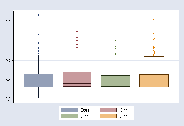
Simulate three datasets using gllasim and obtain empirical Bayes predictions for Figure 9.2 (output not shown)
set seed 1322411
matrix aa=e(b)
gllasim y, from(aa)
gllamm y age xero cosine sine female height stunted, i(id) l(logit) f(binom) nip(12) from(aa) copy adapt
gllapred SIM1, u
drop y
gllasim y, from(aa)
gllamm y age xero cosine sine female height stunted, i(id) l(logit) f(binom)  nip(12) from(aa) copy adapt
gllapred SIM2, u
drop y
gllasim y, from(aa)
gllamm y age xero cosine sine female height stunted, i(id) l(logit) f(binom) nip(12) from(aa) copy adapt
gllapred SIM3, u
drop y
Make Figure 9.2 and store as ichs2.gph (note that simulated datasets are different due to different seed)
graph box ebm1 SIM1m1 SIM2m1 SIM3m1 if last==1, t2(" ") saving(ichs2, replace) /*
  */ legend(lab(1 "Data") lab(2 "Sim 1") lab(3 "Sim 2") lab(4 "Sim 3") ) /*
  */ marker(1, m(oh)) marker(2, m(oh)) marker(3, m(oh)) marker(4, m(oh)) lintensity(255)
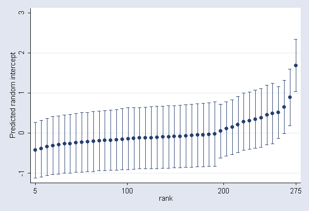
Make Figure 9.3 and store as ichs3.gph
sort ebm1
gen rank = sum(last)
serrbar ebm1 ebs1 rank if last==1&mod(rank,6)==5, xlab(5 100 200 275)  /*
  */ ytitle("Predicted random intercept") saving(ichs3, replace)
Create small dataset with covariate values for which we want predictions for Figure 9.1
keep in 1/83
replace age = -32+_n-1
replace cosine=-1
replace sine= 0
replace xero=0
replace female=1
summ height
replace height=r(mean)
replace stunted=0
gen y=1
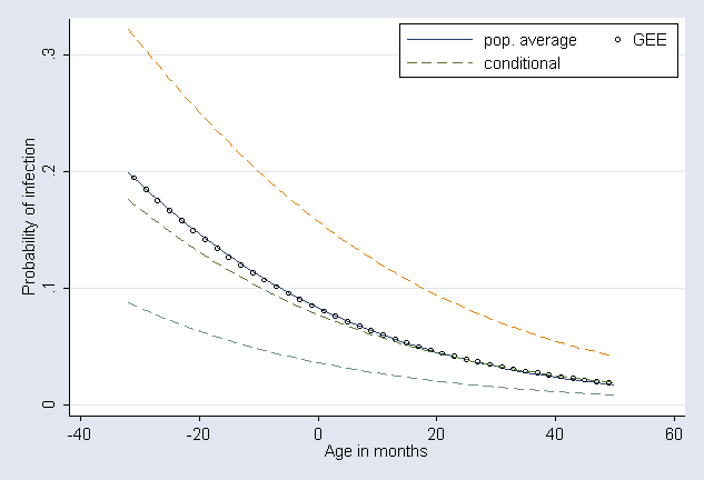
Obtain marginal and conditional probabilities for random intercept model using gllapred
gllapred mu_m, mu marg from(aa)
gen u01=0
gen u8p1 = 0.8
gen u8m1 = -0.8
gllapred mu_0, mu us(u0)
gllapred mu_8p, mu us(u8p)
gllapred mu_8m, mu us(u8m)
Obtain marginal probabilities for GEE by restoring the stored estimates using _estimates unhold and using Stata's predict command.
_estimates unhold gee
predict mu_g, mu
label variable mu_g "GEE"
label variable mu_0 "u=0"
label variable mu_8p "u=+0.8"
label variable mu_8m "u=-0.8"
label variable mu_m "pop. average"
Make Figure 9.1 (ichs.gph)
sort age
twoway (line mu_m age, clpatt(solid)) /*
  */ (scatter mu_g age if mod(age,2)==1, ms(oh) mc(black)) (line mu_0 age, clpatt(dash)) /*
  */ (line mu_8p age, clpatt(dash)) (line mu_8m age, clpatt(dash)), /*
  */ legend(order(1 2 3) label(3 "conditional") position(1) ring(0) ) /*
  */ ytitle("Probability of infection") /*
  */ xtitle("Age in months") saving(ichs, replace)
Zeger, S. L. and Karim, M. R. (1991). Generalized linear models with random effects: A Gibbs sampling approach. Journal of the American Statistical Association 86, 79-86.
Diggle, P. J., Heagerty, P. J., Liang, K.-Y. and Zeger, S. L. (2002). Analysis of Longitudinal Data. Oxford: Oxford University Press.
Rabe-Hesketh, S., Skrondal, A. and Pickles, A. (2002). Reliable estimation of generalised linear mixed models using adaptive quadrature. The Stata Journal 2, 1-21.
Skrondal, A. and Rabe-Hesketh, S. (2004). Generalized
Latent Variable Modeling: Multilevel, Longitudinal and Structural
Equation Models. Boca Raton, FL: Chapman & Hall/ CRC Press.
Outline
Datasets and do-files