The data set used in this section is mislevy.dat. Below we assume that this has been saved in the current directory.
The do-file is mislevy.do.
The programs we use are gllamm and gllapred. You can find the programs and download them by issuing the command findit gllamm and findit gllapred. For more information see http://www.gllamm.org.
Read and prepare the data
insheet using mislevy.dat, clear
list, clean
       y1   y2   y3   y4   cwm   cwf   cbm   cbf
  1.    0    0    0    0    23    20    27    29
  2.    0    0    0    1     5     8     5     8
  3.    0    0    1    0    12    14    15     7
  4.    0    0    1    1     2     2     3     3
  5.    0    1    0    0    16    20    16    14
  6.    0    1    0    1     3     5     5     5
  7.    0    1    1    0     6    11     4     6
  8.    0    1    1    1     1     7     3     0
  9.    1    0    0    0    22    23    15    14
 10.    1    0    0    1     6     8    10    10
 11.    1    0    1    0     7     9     8    11
 12.    1    0    1    1    19     6     1     2
 13.    1    1    0    0    21    18     7    19
 14.    1    1    0    1    11    15     9     5
 15.    1    1    1    0    23    20    10     8
 16.    1    1    1    1    86    42     2     4
Stack variables cwm, cwf, cbm and cbf into a single frequency variable wt2 and create dummies w for white and m for male
gen i=_n
reshape long cw cb,i(i) j(male) string
replace i=_n
reshape long c, i(i) j(white) string
drop i

encode white, gen(w)
encode male, gen(m)
replace w=w-1
replace m=m-1

rename c wt2
list in 1/10, clean nolab

       white   male   y1   y2   y3   y4   wt2   w   m
  1.       b      f    0    0    0    0    29   0   0
  2.       w      f    0    0    0    0    20   1   0
  3.       b      m    0    0    0    0    27   0   1
  4.       w      m    0    0    0    0    23   1   1
  5.       b      f    0    0    0    1     8   0   0
  6.       w      f    0    0    0    1     8   1   0
  7.       b      m    0    0    0    1     5   0   1
  8.       w      m    0    0    0    1     5   1   1
  9.       b      f    0    0    1    0     7   0   0
 10.       w      f    0    0    1    0    14   1   0
Calculate tot, the sizes of the four groups defined by w and m
egen tot = sum(wt2), by(w m)
Stack responses y1 to y4 into a single vector and create variable item
gen patt=_n
reshape long y, i(patt) j(item)
list in 1/8, clean nolab

       patt   item   white   male   y   wt2   w   m
  1.      1      1       b      f   0    29   0   0
  2.      1      2       b      f   0    29   0   0
  3.      1      3       b      f   0    29   0   0
  4.      1      4       b      f   0    29   0   0
  5.      2      1       w      f   0    20   1   0
  6.      2      2       w      f   0    20   1   0
  7.      2      3       w      f   0    20   1   0
  8.      2      4       w      f   0    20   1   0
Create dummy variables d1 to d4 for items 1 to 4
qui tab item, gen(d)
Estimate the one-parameter logistic IRT model (Table 9.5)
gllamm y d1 d2 d3 d4, i(patt) l(logit) f(binom) weight(wt) nocons adapt


number of level 1 units = 3104
number of level 2 units = 776

Condition Number = 1.6838733

gllamm model

log likelihood = -2004.9379

------------------------------------------------------------------------------
           y |      Coef.   Std. Err.      z    P>|z|     [95% Conf. Interval]
-------------+----------------------------------------------------------------
          d1 |   .5775969   .0969974     5.95   0.000     .3874854    .7677083
          d2 |   .2382793   .0950415     2.51   0.012     .0520014    .4245572
          d3 |  -.2247582   .0949752    -2.37   0.018    -.4109062   -.0386102
          d4 |  -.5938583   .0971079    -6.12   0.000    -.7841863   -.4035303
------------------------------------------------------------------------------


Variances and covariances of random effects
------------------------------------------------------------------------------


***level 2 (patt)

    var(1): 1.6285398 (.20840709)
------------------------------------------------------------------------------
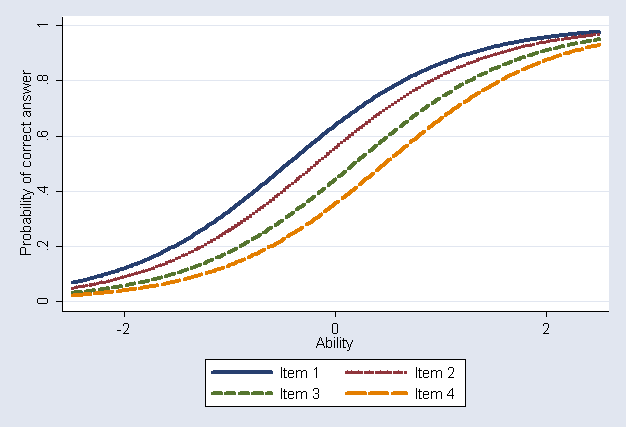
Plot the item characteristic curves (Figure 9.5)
matrix list e(b)

e(b)[1,5]
             y:          y:          y:          y:      patt1:
            d1          d2          d3          d4       _cons
y1   .57759686   .23827933  -.22475821  -.59385829   1.2761425

twoway (function y=1/(1+exp(-[y]d1 -x*[patt1]_cons)), range(-2.5 2.5))                   /*
*/     (function y=1/(1+exp(-[y]d2 -x*[patt1]_cons)), range(-2.5 2.5) clpatt(dot))       /*
*/     (function y=1/(1+exp(-[y]d3 -x*[patt1]_cons)), range(-2.5 2.5) clpatt(dash))      /*
*/     (function y=1/(1+exp(-[y]d4 -x*[patt1]_cons)), range(-2.5 2.5) clpatt(longdash)), /*
*/     legend( label(1 "Item 1") label(2 "Item 2") label(3 "Item 3") label(4 "Item 4") ) /*
*/     xtitle(Ability) ytitle(Probability of correct answer)
eq load: d1-d4
gllamm y d1-d4, i(patt) eqs(load) l(logit) f(binom) weight(wt) nocons adapt nip(12)

number of level 1 units = 3104
number of level 2 units = 776

Condition Number = 5.4532607

gllamm model

log likelihood = -2002.7391

------------------------------------------------------------------------------
           y |      Coef.   Std. Err.      z    P>|z|     [95% Conf. Interval]
-------------+----------------------------------------------------------------
          d1 |   .6453275   .1206319     5.35   0.000     .4088932    .8817617
          d2 |   .2194106   .0890237     2.46   0.014     .0449274    .3938939
          d3 |  -.2156426   .0908816    -2.37   0.018    -.3937672    -.037518
          d4 |  -.6251801    .109345    -5.72   0.000    -.8394923   -.4108678
------------------------------------------------------------------------------


Variances and covariances of random effects
------------------------------------------------------------------------------


***level 2 (patt)

    var(1): 2.6007398 (.87041805)

    loadings for random effect 1
    d1: 1 (fixed)
    d2: .64650121 (.15490565)
    d3: .69484866 (.16864938)
    d4: .89729467 (.21828051)

------------------------------------------------------------------------------
The variance and factor loading estimates differ a little from those in Table 9.5.
Plot item characteristic curves (Figure 9.5)
matrix list e(b)

e(b)[1,8]
             y:          y:          y:          y:    pat1_1l:    pat1_1l:    pat1_1l:
            d1          d2          d3          d4          d2          d3          d4
y1   .64532747   .21941063  -.21564261  -.62518007   .64650121   .69484866   .89729467

        pat1_1:
            d1
y1   1.6126809

twoway (function y=1/(1+exp(-[y]d1 -x*[pat1_1]d1)), range(-2.5 2.5))                               /*
*/     (function y=1/(1+exp(-[y]d2 -x*[pat1_1]d1*[pat1_1l]d2)), range(-2.5 2.5) clpatt(dot))       /*
*/     (function y=1/(1+exp(-[y]d3 -x*[pat1_1]d1*[pat1_1l]d3)), range(-2.5 2.5) clpatt(dash))      /*
*/     (function y=1/(1+exp(-[y]d4 -x*[pat1_1]d1*[pat1_1l]d4)), range(-2.5 2.5) clpatt(longdash)), /*
*/     legend( label(1 "Item 1") label(2 "Item 2") label(3 "Item 3") label(4 "Item 4") )           /*
*/     xtitle(Ability) ytitle(Probability of correct answer)
Estimate two-parameter IRT model with non-zero mean ability, setting the item difficulty of item 1 to zero (Table 9.6)
gen cons=1
eq load: d1-d4
eq f1: cons

gllamm y d2-d4, i(patt) eqs(load) l(logit) f(binom) weight(wt) /*
   */ geqs(f1) nocons adapt nip(12)

number of level 1 units = 3104
number of level 2 units = 776

Condition Number = 6.9163564

gllamm model

log likelihood = -2002.7391

------------------------------------------------------------------------------
           y |      Coef.   Std. Err.      z    P>|z|     [95% Conf. Interval]
-------------+----------------------------------------------------------------
          d2 |   -.197791   .1174163    -1.68   0.092    -.4279228    .0323408
          d3 |  -.6640437   .1352743    -4.91   0.000    -.9291764    -.398911
          d4 |  -1.204219   .1846912    -6.52   0.000    -1.566207   -.8422309
------------------------------------------------------------------------------


Variances and covariances of random effects
------------------------------------------------------------------------------


***level 2 (patt)

    var(1): 2.6008217 (.87044376)

    loadings for random effect 1
    d1: 1 (fixed)
    d2: .64648882 (.15490305)
    d3: .69483564 (.1686465)
    d4: .89727244 (.21827359)


Regressions of latent variables on covariates
------------------------------------------------------------------------------


    random effect 1 has 1 covariates:
    cons: .64533407 (.12063317)
------------------------------------------------------------------------------
The estimates differ a little from those in Table 9.6.
Empirical Bayes predictions: EAP ability scores
gllapred IRT, fac

(means and standard deviations will be stored in IRTm1 IRTs1)
Estimate a MIMIC model where ability depends on sex (dummy f), race (dummy b) and their interaction (Table 9.6)
gen f=1-m
gen b=1-w
gen b_f = b*f
eq f1: cons f b b_f
matrix a=e(b)
gllamm y d2-d4, i(patt) eqs(load) l(logit) f(binom) weight(wt) /*
  */ geqs(f1) from(a) nocons adapt nip(12)

number of level 1 units = 3104
number of level 2 units = 776

Condition Number = 10.407055

gllamm model

log likelihood = -1956.2333

------------------------------------------------------------------------------
           y |      Coef.   Std. Err.      z    P>|z|     [95% Conf. Interval]
-------------+----------------------------------------------------------------
          d2 |  -.2114786   .1159544    -1.82   0.068    -.4387451     .015788
          d3 |  -.7145968   .1379683    -5.18   0.000    -.9850096   -.4441839
          d4 |  -1.159195   .1601593    -7.24   0.000    -1.473101   -.8452882
------------------------------------------------------------------------------


Variances and covariances of random effects
------------------------------------------------------------------------------


***level 2 (patt)

    var(1): 1.9689171 (.60516363)

    loadings for random effect 1
    d1: 1 (fixed)
    d2: .67658546 (.14380046)
    d3: .77264707 (.16674369)
    d4: .86240868 (.17342379)


Regressions of latent variables on covariates
------------------------------------------------------------------------------


    random effect 1 has 4 covariates:
    cons: 1.4345373 (.21553973)
    f: -.6200911 (.20526977)
    b: -1.6843558 (.31129702)
    b_f: .67057381 (.32116754)
------------------------------------------------------------------------------
The estimates differ a little from those in Table 9.6.
Empirical Bayes predictions: EAP ability scores
gllapred MIMIC, fac

(means and standard deviations will be stored in MIMICm1 MIMICs1)
Look at ability scores for each response and covariate pattern (Table 9.7)
drop d1-d4
reshape wide y, i(patt) j(item)
sort y1-y4 b f
list y1-y4 b f IRTm1 MIMICm1, nolab clean

       y1   y2   y3   y4   b   f        IRTm1      MIMICm1
  1.    0    0    0    0   0   0   -1.2242641   -.55473277
  2.    0    0    0    0   0   1   -1.2242641   -.87608943
  3.    0    0    0    0   1   0   -1.2242641   -1.4707461
  4.    0    0    0    0   1   1   -1.2242641   -1.4410752
  5.    0    0    0    1   0   0      -.14876    .26704248
  6.    0    0    0    1   0   1      -.14876   -.02615521
  7.    0    0    0    1   1   0      -.14876   -.54782301
  8.    0    0    0    1   1   1      -.14876   -.52233467
  9.    0    0    1    0   0   0   -.37675812    .18398721
 10.    0    0    1    0   0   1   -.37675812   -.11085131
 11.    0    0    1    0   1   0   -.37675812   -.63777142
 12.    0    0    1    0   1   1   -.37675812    -.6119613
 13.    0    0    1    1   0   0    .60364936    .97836482
 14.    0    0    1    1   0   1    .60364936    .68778691
 15.    0    0    1    1   1   0    .60364936    .19041653
 16.    0    0    1    1   1   1    .60364936    .21416676
 17.    0    1    0    0   0   0   -.43218061    .09469579
 18.    0    1    0    0   0   1   -.43218061   -.20221901
 19.    0    1    0    0   1   0   -.43218061   -.73534825
 20.    0    1    0    0   1   1   -.43218061   -.70916483
 21.    0    1    0    1   0   0    .55196233     .8893892
 22.    0    1    0    1   0   1    .55196233    .59958378
 23.    0    1    0    1   1   0    .55196233    .10115863
 24.    0    1    0    1   1   1    .55196233    .12502831
 25.    0    1    1    0   0   0    .33515561    .80656055
 26.    0    1    1    0   0   1    .33515561    .51719789
 27.    0    1    1    0   1   0    .33515561    .01729505
 28.    0    1    1    0   1   1    .33515561     .0413004
 29.    0    1    1    1   0   0    1.3035676    1.6228636
 30.    0    1    1    1   0   1    1.3035676    1.3180372
 31.    0    1    1    1   1   0    1.3035676    .81295145
 32.    0    1    1    1   1   1    1.3035676    .83659008
 33.    1    0    0    0   0   0    -.0351866     .3938274
 34.    1    0    0    0   0   1    -.0351866    .10259226
 35.    1    0    0    0   1   0    -.0351866   -.41203827
 36.    1    0    0    0   1   1    -.0351866   -.38699316
 37.    1    0    0    1   0   0    .93089004    1.1908602
 38.    1    0    0    1   0   1    .93089004    .89722329
 39.    1    0    0    1   1   0    .93089004    .40020559
 40.    1    0    0    1   1   1    .93089004    .42377722
 41.    1    0    1    0   0   0    .71352262    1.1065918
 42.    1    0    1    0   0   1    .71352262    .81436966
 43.    1    0    1    0   1   0    .71352262    .31757081
 44.    1    0    1    0   1   1    .71352262    .34119563
 45.    1    0    1    1   0   0    1.7045824    1.9484446
 46.    1    0    1    1   0   1    1.7045824    1.6312163
 47.    1    0    1    1   1   0    1.7045824     1.113084
 48.    1    0    1    1   1   1    1.7045824    1.1371117
 49.    1    1    0    0   0   0    .66179647    1.0169609
 50.    1    1    0    0   0   1    .66179647    .72595346
 51.    1    1    0    0   1   0    .66179647    .22887171
 52.    1    1    0    0   1   1    .66179647    .25257845
 53.    1    1    0    1   0   0    1.6485285    1.8501881
 54.    1    1    0    1   0   1    1.6485285    1.5370316
 55.    1    1    0    1   1   0    1.6485285    1.0234149
 56.    1    1    0    1   1   1    1.6485285    1.0472972
 57.    1    1    1    0   0   0    1.4181578    1.7596042
 58.    1    1    1    0   0   1    1.4181578    1.4499547
 59.    1    1    1    0   1   0    1.4181578     .9400666
 60.    1    1    1    0   1   1    1.4181578    .96383584
 61.    1    1    1    1   0   0     2.506591    2.6876937
 62.    1    1    1    1   0   1     2.506591    2.3322937
 63.    1    1    1    1   1   0     2.506591    1.7665629
 64.    1    1    1    1   1   1     2.506591    1.7923462
The scores differ a little from those in Table 9.7.
Mislevy, R. J. (1985). Estimation of latent group effects. Journal of the American Statistical Association 80, 993-997.
Skrondal, A. and Rabe-Hesketh, S. (2004). Generalized
Latent Variable Modeling: Multilevel, Longitudinal and Structural
Equation Models. Boca Raton, FL: Chapman & Hall/ CRC Press.
Outline
Datasets and do-files
