The data set used in this section is gum.dat from Silagy (2003).
The do-file is gum.do.
The programs used are gllamm and gllapred. Use the command ssc describe gllamm and follow instructions to download these GLLAMM commands. For more information on GLLAMM see http://www.gllamm.org.
Read and list data:
insheet using gum.dat, clear
rename study studynam
gen study=_n
list, clean

              studynam    d1    n1    d0    n0   study
  1.      Blondal 1989    37    92    24    90       1
  2.     Campbell 1991    21   107    21   105       2
  3.   Fagerstrom 1982    30    50    23    50       3
  4.          Fee 1982    23   180    15   172       4
  5.       Garcia 1989    21    68     5    38       5
  6.       Garvey 2000    75   405    17   203       6
  7.        Gross 1995    37   131     6    46       7
  8.         Hall 1985    18    41    10    36       8
  9.         Hall 1987    30    71    14    68       9
 10.         Hall 1996    24    98    28   103      10
 11.   Hjalmarson 1984    31   106    16   100      11
 12.        Huber 1988    31    54    11    60      12
 13.       Jarvis 1982    22    58     9    58      13
 14.       Jensen 1991    90   211    28    82      14
 15.       Killen 1984    16    44     6    20      15
 16.       Killen 1990   129   600   112   617      16
 17.      Malcolm 1980     6    73     3   121      17
 18.     McGovern 1992    51   146    40   127      18
 19.     Nakamura 1990    13    30     5    30      19
 20.       Niaura 1994     5    84     4    89      20
 21.       Niaura 1999     1    31     2    31      21
 22.        Pirie 1992    75   206    50   211      22
 23.        Puska 1979    29   116    21   113      23
 24.    Schneider 1985     9    30     6    30      24
 25.     Tonnesen 1988    23    60    12    53      25
 26.        Villa 1999    11    21    10    26      26
 27.       Zelman 1992    23    58    18    58      27
Prepare data for analysis, creating variables
gum=1 if in treatment arm, 0 otherwise
quit=1 if quit smoking, 0 otherwise
wt1: frequency weight
reshape long d n, i(study) j(gum)

(note: j = 0 1)

Data                               wide   ->   long
-----------------------------------------------------------------------------
Number of obs.                       27   ->      54
Number of variables                   6   ->       5
j variable (2 values)                     ->   gum
xij variables:
                                  d0 d1   ->   d
                                  n0 n1   ->   n
-----------------------------------------------------------------------------

gen y0 = n-d
rename d y1
gen i=_n
reshape long y, i(i) j(quit)

(note: j = 0 1)

Data                               wide   ->   long
-----------------------------------------------------------------------------
Number of obs.                       54   ->     108
Number of variables                   7   ->       7
j variable (2 values)                     ->   quit
xij variables:
                                  y0 y1   ->   y
-----------------------------------------------------------------------------

drop i
rename y wt1


sort study gum quit
list in 1/12, clean

       quit   study   gum          studynam   wt1     n
  1.      0       1     0      Blondal 1989    66    90
  2.      1       1     0      Blondal 1989    24    90
  3.      0       1     1      Blondal 1989    55    92
  4.      1       1     1      Blondal 1989    37    92
  5.      0       2     0     Campbell 1991    84   105
  6.      1       2     0     Campbell 1991    21   105
  7.      0       2     1     Campbell 1991    86   107
  8.      1       2     1     Campbell 1991    21   107
  9.      0       3     0   Fagerstrom 1982    27    50
 10.      1       3     0   Fagerstrom 1982    23    50
 11.      0       3     1   Fagerstrom 1982    20    50
 12.      1       3     1   Fagerstrom 1982    30    50
Continuous random intercept and slope model for Table 9.9 using gllamm (iteration log not shown):
gen treat = gum -0.5
gen cons=1
eq int: cons
eq slop: treat


gllamm quit treat, i(study) nrf(2) eqs(int slop) l(logit) /*
  */ f(binom) weight(wt) adapt nocor trace allc

number of level 1 units = 5908
number of level 2 units = 27

Condition Number = 1.7685027

gllamm model

log likelihood = -3074.1459

------------------------------------------------------------------------------
        quit |      Coef.   Std. Err.      z    P>|z|     [95% Conf. Interval]
-------------+----------------------------------------------------------------
       treat |   .5670943   .0881729     6.43   0.000     .3942786      .73991
       _cons |    -1.1658   .1401855    -8.32   0.000    -1.440559   -.8910418
------------------------------------------------------------------------------


Variances and covariances of random effects
------------------------------------------------------------------------------


***level 2 (study)

    var(1): .48050074 (.15333759)
    cov(2,1): fixed at 0

    var(2): .05190697 (.04639595)
------------------------------------------------------------------------------


------------------------------------------------------------------------------
        quit |      Coef.   Std. Err.      z    P>|z|     [95% Conf. Interval]
-------------+----------------------------------------------------------------
quit         |
       treat |   .5670943   .0881729     6.43   0.000     .3942786      .73991
       _cons |    -1.1658   .1401855    -8.32   0.000    -1.440559   -.8910418
-------------+----------------------------------------------------------------
stu1_1       |
        cons |   .6931816   .1106042     6.27   0.000     .4764014    .9099619
-------------+----------------------------------------------------------------
stu1_2       |
       treat |    .227831    .101821     2.24   0.025     .0282656    .4273964
------------------------------------------------------------------------------
Slight discrepancy for the treatment effect standard deviation disappears when nip(20) is used.
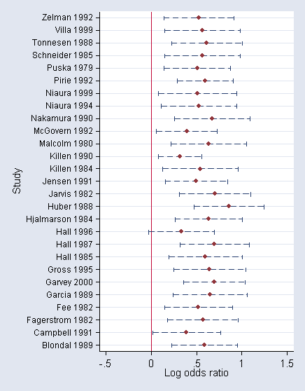
Empirical Bayes predictions of study-specific effect sizes using gllapred:
gllapred eff, u

(means and standard deviations will be stored in effm1 effs1 effm2 effs2)
Non-adaptive log-likelihood: -3078.3785
-3101.5793 -3092.8436 -3088.3938 -3084.9338 -3081.8962 -3079.2417
-3077.5891 -3076.3852 -3074.9084 -3074.1634 -3074.1459 -3074.1459
log-likelihood:-3074.1459
95% intervals
gen eff = effm2 + _b[treat]
gen lower = effm2 + _b[treat] - 1.96*effs2
gen upper = effm2 + _b[treat] + 1.96*effs2
List results:
sort study
qui by study: gen last=_n==_N
list studynam lower eff upper if last==1, clean

              studynam       lower        eff      upper
  4.      Blondal 1989     .222363   .5866519   .9509408
  8.     Campbell 1991    .0146321   .3882984   .7619646
 12.   Fagerstrom 1982    .1783771   .5678892   .9574013
 16.          Fee 1982    .1462535   .5193934   .8925332
 20.       Garcia 1989    .2424062   .6489648   1.055523
 24.       Garvey 2000    .3575259   .6972256   1.036925
 28.        Gross 1995    .2477593   .6437063   1.039653
 32.         Hall 1985      .19287   .5980018   1.003134
 36.         Hall 1987    .3139485   .6961169   1.078285
 40.         Hall 1996   -.0332232   .3325011   .6982254
 44.   Hjalmarson 1984     .259717   .6314499   1.003183
 48.        Huber 1988    .4692236   .8577137   1.246204
 52.       Jarvis 1982    .3085245   .7037886   1.099053
 56.       Jensen 1991    .1502759   .4940711   .8378663
 60.       Killen 1984    .1223252   .5393925   .9564598
 64.       Killen 1990    .0739083   .3133026   .5526969
 68.      Malcolm 1980    .2148292   .6320365   1.049244
 72.     McGovern 1992    .0535688   .3903244   .7270799
 76.     Nakamura 1990    .2542217   .6702684   1.086315
 80.       Niaura 1994    .1086343   .5270553   .9454764
 84.       Niaura 1999    .0755295   .5087444   .9419592
 88.        Pirie 1992    .2841303   .5926718   .9012133
 92.        Puska 1979     .139473   .5054876    .871502
 96.    Schneider 1985    .1465653   .5650316    .983498
100.     Tonnesen 1988    .2204977   .6133725   1.006247
104.        Villa 1999    .1476256   .5656016   .9835777
108.       Zelman 1992    .1351462    .522485   .9098238
Plot results using forest plot (similar to Figure 9.6):
encode studynam, gen(s)
twoway (rcap lower upper s, horizontal blpattern(dash)) (scatter s eff),   /*
  */ ylabel(1(1)27,valuelabels angle(horizontal) labs(small)) legend(off)  /*
  */ xscale(range(-.5 1.5)) ysize(7) xlab(-.5(.5)1.5) xline(0) saving(gumf)
Nonoarametric maximum likelihood (NPML) estimates using gateaux derivative:
Start with two masses (iteration log not shown):
gllamm quit treat, i(study) nrf(2) eqs(int slop) l(logit) /*
  */ f(binom) weight(wt) ip(f) nip(2)

number of level 1 units = 5908
number of level 2 units = 27

Condition Number = 12.81975

gllamm model

log likelihood = -3106.6101

------------------------------------------------------------------------------
        quit |      Coef.   Std. Err.      z    P>|z|     [95% Conf. Interval]
-------------+----------------------------------------------------------------
       treat |   .5317816   .0666912     7.97   0.000     .4010692     .662494
       _cons |  -1.086669   .0919203   -11.82   0.000    -1.266829   -.9065085
------------------------------------------------------------------------------


Probabilities and locations of random effects
------------------------------------------------------------------------------


***level 2 (study)

    loc1: -.53793, .35823
  var(1): .19270432

    loc2: -.09286, .06184
cov(2,1): .03326538
  var(2): .0057424
    prob: 0.3997, 0.6003
------------------------------------------------------------------------------
Add one mass at a time using gateaux derivative method (output not shown):
local n=2
while $HG_error==0&`n'<12{
    matrix a = e(b)
    local ll = e(ll)
    local k = e(k)
    local n = `n' + 1
    gllamm quit treat , i(study) nrf(2) eqs(int slop) l(logit) /*
       */ f(binom) weight(wt) ip(f) nip(`n') lf0(`k' `ll') /*
       */ gateaux(-5 5 40) from(a) trace
 }
Final estimates for 10 masses:
number of level 1 units = 5908
number of level 2 units = 27
Condition Number = 111.7378
gllamm model Number of obs = 5908
LR chi2(3) = 0.36
Log likelihood = -3061.5044 Prob > chi2 = 0.9488
------------------------------------------------------------------------------
quit | Coef. Std. Err. z P>|z| [95% Conf. Interval]
-------------+----------------------------------------------------------------
treat | .5909019 .1020571 5.79 0.000 .3908736 .7909301
_cons | -1.197405 .1530979 -7.82 0.000 -1.497471 -.8973385
------------------------------------------------------------------------------
Probabilities and locations of random effects
------------------------------------------------------------------------------
***level 2 (study)
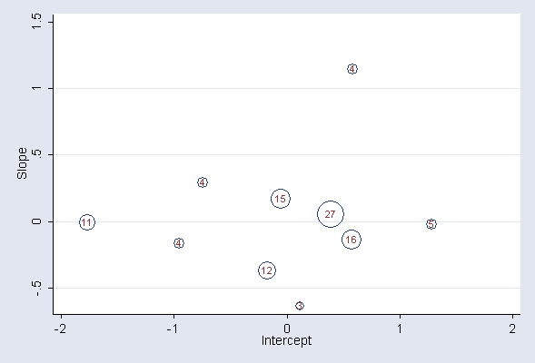
loc1: -.17192, -1.7707, -.74877, 1.2864, .58648, -.05122, .11831, -.95241, .57538, .39284
var(1): .57783952
loc2: -.37184, -.0051, .28878, -.02044, 1.1465, .16963, -.63535, -.16783, -.13978, .05351
cov(2,1): .01816208
var(2): .09297283
prob: 0.1216, 0.106, 0.0442, 0.0461, 0.0382, 0.1482, 0.0325, 0.0355, 0.1617, 0.2662
------------------------------------------------------------------------------
Store locations and log odds as variables:
matrix a=e(zlc2)'
svmat a
matrix b=e(zlc3)'
svmat b
matrix prob = e(zps2)'
svmat prob
Convert log odds to probabilities and calculate corresponding rounded percentages:
replace prob1=exp(prob1)
gen percent=round(prob1*100,1)
Produce a plot similar to the upper panel of Figure 9.7:
twoway (scatter b1 a1 [w=percent], msymbol(Oh))   /*
  */ (scatter b1 a1, mlabel(percent) mlabpos(0) msymbol(none)), /*
  */ xtitle(Intercept) ytitle(Slope) legend(off) saving(blobs, replace)
Silagy, C. (2003). Nicotine replacement therapy for smoking cessation (Cochrane review). The Cochrane Library, Issue 4. Chichester: Wiley.
Rabe-Hesketh, S., Skrondal, A. and Pickles, A. (2002). Reliable estimation of generalised linear mixed models using adaptive quadrature. The Stata Journal 2, 1-21.
Skrondal, A. and Rabe-Hesketh, S. (2004). Generalized
Latent Variable Modeling: Multilevel, Longitudinal and Structural
Equation Models. Boca Raton, FL: Chapman & Hall/ CRC Press.
Outline
Datasets and do-files