The data set used in this section is wjobs.dat. We would like to thank Amiram Vinokur and Bengt Muthén for making the data available.
The do-file is cace.do.
The program used is gllamm. Use the command ssc describe gllamm and follow instructions to download gllamm. For more information on gllamm see http://www.gllamm.org.
| depress | depression (response variable) |
| risk | baseline risk score |
| Tx | randomized to receive job training (1:yes, 0:no). This is r_j |
| basedep | baseline depression score |
| age | age in years |
| motivate | motivation to attend training |
| educ | school grade completed |
| assert | assertiveness |
| single | dummy for being single |
| econ | economic hardship |
| nonwhite | dummy for not being white |
| x10 | not used |
| c1 | complier in treatment group (1: complied, 0: did not comply). This is c_j |
| c2 | not used |
Read and prepare data
infile depress risk r depbase age motivate educ /*
   */ assert single econ nonwhite x10 c c0 using wjobs.dat, clear


gen y1 = c if r==1  /* compliance missing in control group */
gen y2 = depress


gen id=_n
reshape long y, i(id) j(var)
drop if y==.
tab var, gen(d)     /* create dummies d1 and d2 */
List some data
list id var d1 d2 y r c if id==1 | id==2 | id==175 | id==176, clean

        id   var   d1   d2       y   r   c
  1.     1     2    0    1     .45   0   1
  2.     2     2    0    1    -.72   0   1
182.   175     1    1    0       0   1   0
183.   175     2    0    1   -1.37   1   0
184.   176     1    1    0       1   1   1
185.   176     2    0    1     .54   1   1
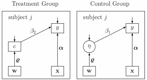
Path diagram of CACE model
Interactions and equations (for model without covariates)
gen nr_d2 = (1-r)*d2
gen c_r_d2 = c*r*d2


eq load: nr_d2         /* for beta_1(1-r_j)d_2i */
Constraints
cons def 1 [p2_1]_cons = [y]d1    /* constraint for varrho */
cons def 2 [z2_1_1]nr_d2 = 1      /* e_1 = 1 */
cons def 3 [z2_1_2]nr_d2 = 0      /* e_2 = 0 */
gllamm command for model without covariates in Table 14.6 (iteration log not shown)
gllamm y d1 d2 c_r_d2, i(id) eqs(load) l(logit ident) /*
  */ f(binom gauss) lv(var) fv(var) ip(fn) nip(2)     /*
  */ constr(1/3) frload(1) nocons     /* beta_1 is "freed" by frload(1) */

number of level 1 units = 837
number of level 2 units = 502

Condition Number = 5.8885922

gllamm model with constraints:
 ( 1) - [y]d1 + [p2_1]_cons = 0
 ( 2)  [z2_1_1]nr_d2 = 1
 ( 3)  [z2_1_2]nr_d2 = 0

log likelihood = -815.1493933028294

------------------------------------------------------------------------------
             |      Coef.   Std. Err.      z    P>|z|     [95% Conf. Interval]
-------------+----------------------------------------------------------------
          d1 |   .1855983   .1097431     1.69   0.091    -.0294942    .4006907
          d2 |  -.3909498   .0651724    -6.00   0.000    -.5186854   -.2632143
      c_r_d2 |  -.1224928   .0867746    -1.41   0.158    -.2925679    .0475822
------------------------------------------------------------------------------

Variance at level 1
------------------------------------------------------------------------------

  .60067675 (.03791846)

Probabilities and locations of random effects
------------------------------------------------------------------------------


***level 2 (id)

    loc1: 1, 0
  var(1): .24785938

    loadings for random effect 1
    nr_d2: .01526969 (.17004298)

    prob: 0.5463, 0.4537
------------------------------------------------------------------------------
Estimate of Complier average causal effect:
lincom [y]c_r_d2 - [id1_1l]nr_d2

 ( 1)  [y]c_r_d2 - [id1_1l]nr_d2 = 0

------------------------------------------------------------------------------
           y |      Coef.   Std. Err.      z    P>|z|     [95% Conf. Interval]
-------------+----------------------------------------------------------------
         (1) |  -.1377625    .141096    -0.98   0.329    -.4143056    .1387806
------------------------------------------------------------------------------
Define more interactions to add covariates to the model
Make interactions with d1 (dummy for compliance response), for compliance model
gen age_d1 = age*d1
gen motivate_d1 = motivate*d1
gen educ_d1 = educ*d1
gen assert_d1 = assert*d1
gen single_d1 = single*d1
gen econ_d1 = econ*d1
gen nonwhite_d1 = nonwhite*d1
Add predictors of depression: make interactions with d2 (dummy for depression response)
gen depbase_d2 = depbase*d2
gen risk_d2 = risk*d2
New constraints: effects of covariates on compliance same in treatment and control groups
cons def 4 [p2_1]age = [y]age_d1
cons def 5 [p2_1]motivate = [y]motivate_d1
cons def 6 [p2_1]educ = [y]educ_d1
cons def 7 [p2_1]assert = [y]assert_d1
cons def 8 [p2_1]single = [y]single_d1
cons def 9 [p2_1]econ = [y]econ_d1
cons def 10 [p2_1]nonwhite = [y]nonwhite_d1
Estimate model with covariates for Table 14.6 using gllamm (iteration log not shown)
eq p: age educ motivate econ assert single nonwhite
eq load: nr_d2
gllamm y d1 age_d1 educ_d1 motivate_d1 econ_d1 assert_d1 single_d1 nonwhite_d1 /*
  */ d2 c_r_d2 depbase_d2 risk_d2, i(id) eqs(load) /*
  */ peqs(p) l(logit ident) f(binom gauss) lv(var) fv(var) ip(fn) nip(2)  /*
  */ constr(1/10) frload(1) nocons

number of level 1 units = 837
number of level 2 units = 502

Condition Number = 508.29708

gllamm model with constraints:
 ( 1) - [y]d1 + [p2_1]_cons = 0
 ( 2)  [z2_1_1]nr_d2 = 1
 ( 3)  [z2_1_2]nr_d2 = 0
 ( 4) - [y]age_d1 + [p2_1]age = 0
 ( 5) - [y]motivate_d1 + [p2_1]motivate = 0
 ( 6) - [y]educ_d1 + [p2_1]educ = 0
 ( 7) - [y]assert_d1 + [p2_1]assert = 0
 ( 8) - [y]single_d1 + [p2_1]single = 0
 ( 9) - [y]econ_d1 + [p2_1]econ = 0
 (10) - [y]nonwhite_d1 + [p2_1]nonwhite = 0

log likelihood = -729.4141540404285

------------------------------------------------------------------------------
             |      Coef.   Std. Err.      z    P>|z|     [95% Conf. Interval]
-------------+----------------------------------------------------------------
          d1 |  -8.740012   1.581554    -5.53   0.000     -11.8398   -5.640222
      age_d1 |   .0790446   .0140223     5.64   0.000     .0515615    .1065277
     educ_d1 |   .2997689   .0675165     4.44   0.000     .1674391    .4320987
 motivate_d1 |   .6668722   .1598218     4.17   0.000     .3536272    .9801172
     econ_d1 |  -.1586014   .1596605    -0.99   0.321    -.4715302    .1543274
   assert_d1 |   -.375871   .1464048    -2.57   0.010    -.6628191   -.0889229
   single_d1 |    .540194   .2754362     1.96   0.050     .0003489    1.080039
 nonwhite_d1 |  -.4985877   .3123484    -1.60   0.110    -1.110779    .1136038
          d2 |   1.632537   .2791255     5.85   0.000     1.085461    2.179613
      c_r_d2 |  -.1299147   .0755598    -1.72   0.086    -.2780092    .0181798
     risk_d2 |   .9117567   .2624528     3.47   0.001     .3973587    1.426155
  depbase_d2 |  -1.463379   .1826867    -8.01   0.000    -1.821438    -1.10532
------------------------------------------------------------------------------

Variance at level 1
------------------------------------------------------------------------------

  .50639704 (.0322776)

Probabilities and locations of random effects
------------------------------------------------------------------------------


***level 2 (id)

    loc1: 1, 0
  var(1): .00016

    loadings for random effect 1
    nr_d2: .1799526 (.1329182)

    prob: 01.6e-04, 0.9998

    log odds parameters
    class 1
    age: .0790446 (.01402225)
    educ: .2997689 (.06751647)
    motivate: .66687221 (.15982181)
    econ: -.15860142 (.15966048)
    assert: -.37587104 (.14640478)
    single: .54019404 (.27543623)
    nonwhite: -.49858773 (.31234837)
    _cons: -8.7400116 (1.5815542)
------------------------------------------------------------------------------
Complier Average Causal Effect
lincom [y]c_r_d2 - [id1_1l]nr_d2

 ( 1)  [y]c_r_d2 - [id1_1l]nr_d2 = 0

------------------------------------------------------------------------------
           y |      Coef.   Std. Err.      z    P>|z|     [95% Conf. Interval]
-------------+----------------------------------------------------------------
         (1) |  -.3098673   .1173219    -2.64   0.008    -.5398141   -.0799205
------------------------------------------------------------------------------
Vinokur, A. D., Price, R. H. and Schul, Y. (1995). Impact of JOBS intervention on unemployed workers varying in risk for depression. American Journal of Community Psychology 19, 543-562.
Little, R. J. A. and Yau, L. H. Y. (1998). Statistical techniques for analyzing data from prevention trials. Psychological Methods 3, 147-159.
Skrondal, A. and Rabe-Hesketh, S. (2004). Generalized
Latent Variable Modeling: Multilevel, Longitudinal and Structural
Equation Models. Boca Raton, FL: Chapman & Hall/ CRC Press.
Outline
Datasets and do-files